This blog entry announces the release of an abstract interpretation-based Ghidra plugin for deobfuscation. The code can be found here (see the ‘Releases’ tab for a binary release). In view of the picture below, the static analysis described herein is designed to take graphs like the one on the left, detect and remove the "opaque predicates" (fake "conditional" branches that only go in one direction), and produce graphs like the one on the right.

Though I have previously published the details of the analysis -- once as a blog post in 2011, once as part of my keynote speech at RECON 2012, entitled "The Case For Semantics-Based Methods in Reverse Engineering" -- the code that I had released at the time was for educational purposes only. It relied upon my private program analysis framework, which was never made public. The current release is fully-functional: you can use it immediately upon installation as an extension in Ghidra. The release ships with a number of examples, which shall be detailed in the rest of this entry. The reader is encouraged to reproduce the results for themselves using the provided scripts and binaries. The code is mostly meant to feed information into larger automated deobfuscation tools, but I have put a good deal of effort into creating user-interactivity and reusable code. I welcome feedback and pull requests for improving my understanding of Ghidra, and also Java development.
Although I prefer my blog entries to be self-contained, given that I've published the details of the analysis already, I don't want to reproduce those details in full. Thus, I shall only sketch the analysis in this entry, and refer the reader to the two links in the previous paragraph should they wish to learn more. (And if you would like to know more about abstract interpretation in general, I published a lengthy introduction to the subject.)
Motivation: Example #1
This example is the obfuscation scenario that lead me to develop this analysis in the first place. Consider the following x86 code, and the annotations off to the right which I created manually:

Through a contorted process, this code pushes the flags onto the stack, and isolates the "TF" bit, also known as the "trap flag", which is set when single-stepping in a debugger. Using a few bitwise operators (AND, OR, and rotations), the code moves the TF bit into the position that the "ZF" bit (the "zero flag") normally occupies, and then loads the flags register with this modified value. Finally, it performs a "JZ" instruction. Since the TF bit has been moved into the ZF position, the JZ is actually testing whether the trap flag had been previously set. If so, the obfuscator corrupts the internal state of the program, leading to a crash later on. This is an anti-debugging mechanism.
The comments to the right demonstrate how I ultimately convinced myself that this was the behavior of the snippet. In essence, we follow the TF bit through the data flow of the code, and ultimately observe that the TF bit governs whether the JZ at the end of the block is taken. We do not know the values of any of the bits labeled "?", but as you can see, we don't need to. Importantly, as with the two AND instructions, we can sometimes determine the values of bits within quantities, even if some of the relevant input bits were unknown to begin with (e.g., notice all the 0 bits produced by the first AND operation above, despite one of the inputs containing 31 "?" bits).
These observations lead me to consider a generic, automated static analysis tool based on the type of analysis just pictured and described. I.e., if I can perform this analysis manually, why can't I write a program to do it for me automatically?
Automating the Analysis
To accomplish that, we will need two ingredients. First, we need to be able to represent quantities within the program (such as the EDX register and the [ESP] memory location) as collections of bits, with the added possibility that we don't know the values of certain bits (namely, the ones marked '?' above). That is to say, we will need to represent bits with three possibilities instead of the normal two: "0", meaning that the bit is known to be zero; "1", similarly with one; and "?" (also written "1/2" in the below), meaning that the bit is unknown. We will call these "three-valued" bits. Furthermore, we will need data structures grouping together fixed-sized collections of three-valued bits, as well as a model of memory containing such quantities.
The second piece that we'll need is the ability to represent the ordinary bitvector operations (such as AND, OR, the rotation operators above, ADD, MUL, IDIV, etc.) for three-valued bits, and do so faithfully with regards to the ordinary two-valued results. That is to say, when the bits are known to be constant, our three-valued operators must behave identically to the two-valued ones. For unknown input bits, the outputs must faithfully capture the results for both possible input values. To illustrate, let's consider the simple example of adapting the ordinary AND operator to the three-valued world. First, recall the ordinary truth table for two-valued AND:

How should AND behave in the presence of unknown bits? That is, what is the value of "0 AND 1/2", "1 AND 1/2", and "1/2 AND 1/2"?
"0 AND 1/2" is easy -- AND only returns 1 if both inputs were 1, so "0 AND 1/2" must be 0.
The "1 AND 1/2" case isn't as nice. Since the "1/2" could represent either 0 or 1, the operation could be either "1 AND 0" (namely, 0) or "1 AND 1" (namely, 1), so we have to say that the result is unknown -- that is to say, "1 AND 1/2" must yield "1/2".
For the same reason, "1/2 AND 1/2" yields "1/2".

As such, the truth table for our three-valued AND is as above. Note that the black values in the corners correspond to the cases when both input bits are known, and that furthermore, they match the two-valued truth table.
In the world of abstract interpretation, an analysis is said to be "correct" if it encompasses all legal data values that may actually occur at runtime. (All abstract interpretation-based analyses are designed to be "correct" by construction.) Since "1/2" refers to any possibility for a given bit, it is always correct for an analysis to decide that a particular output bit is "1/2". Therefore, the red values in the table above could all have been "1/2" (in fact, the black ones could have been "1/2" as well). However, another property of a correct analysis is its "precision". Though harder to quantify, one correct analysis is "more precise" than another if it models fewer data values. Therefore, producing "0" for the "0 AND 1/2" case is both correct (by the analysis above) and more precise than if we'd modeled that case by producing "1/2". Note further in looking at the annotated x86 code above that our choice of modeling 0 AND 1/2 as 0 was crucial in our ability to link the behavior of the JZ instruction at the end to the TF bit at the beginning. Had we modeled 0 AND 1/2 as 1/2 instead, the analysis would have failed to establish that connection.
Similar results may be derived for the other standard bitwise operations:

The OR case works out similarly to the AND case; if an input bit is known to be one, we can use "1" for the output, even if the other bit is unknown. NOT also works out nicely with little imprecision. XOR and == are not so nice; any time an input bit is unknown, the output bit is also unknown.
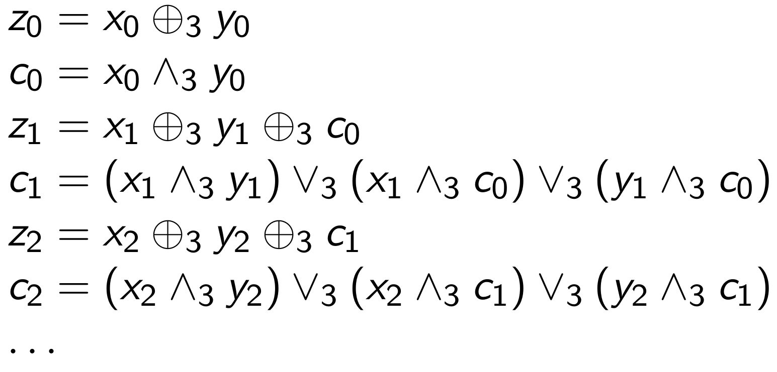
It may be less obvious how to deal with more complicated operations such as addition. The trick lies in realizing that there must be bitwise formulae for computing this operation (since, after all, processors implement these calculations), and we can just use the operators defined above to implement their three-valued counterparts. For example, addition of two quantities "z = x + y" is defined bit-by-bit by the following formulae, where the "c" bits are the carry bits produced at each step in the computation.
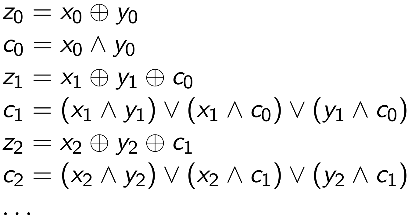
Since we have defined XOR, AND, and OR above, we can simply use the three-valued operators to implement three-valued addition.
The rest of the ordinary bitvector operations -- such as comparisons, shifts (including by unknown amounts), multiplication, and unsigned/signed division and remainder -- can be derived in a similar fashion. If you would like to see more derivations, consult the presentation mentioned previously, and/or read the source code.
Given that the example above writes to (and reads from) the stack, our analysis must also handle memory accesses. We use a crude model wherein only fully-known memory addresses are tracked. Any writes to addresses that are not fully known result in the entire memory state being set to 1/2 (since a write to an unknown destination could overwrite anything). This model is cruder than necessary, and it causes a few complications.
Implementing the Analysis in Ghidra
Since I had previously implemented the analysis for my private framework, my immediate task was simply to port it to Java, and more specifically adapt it to Ghidra's pcode (whereas my prior implementation had targeted my own intermediate representation). First, I needed to familiarize myself with Ghidra pcode. You can enable its display from the Ghidra user interface. After clicking the "Jenga" block in the top-right of the "listing window", right click on "PCode" and select "Enable Field", as below:

Now the listing will display the pcode translations for the assembly instructions:

From here, you can start to get a sense of the pcode language. The Ghidra distribution ships with complete documentation of the pcode language; you can find it in your installation directory under "./docs/languages/index.html".
The initial port was straightforward and took a single day. Noteworthy components of that functionality are:
TVLBitVector.java: implements a class for aggregating fixed numbers of three-valued bits.
TVLBitVectorUtil.java: implements the three-valued version of all supported integer operators, such as AND, addition, etc.
TVLAbstractMemory.java: implements the memory model, associating addresses with TVLBitVector objects.
TVLAbstractGhidraState.java: models the entire state of a Ghidra pcode program: register values, "unique" values, and memory spaces.
TVLAbstractInterpreter.java: the core of the abstract analysis. Given Ghidra pcode objects, query the TVLAbstractGhidraState to obtain the TVLBitVector representations of the inputs, decide which pcode operation is taking place, invoke the relevant method in TVLBitVectorUtil to perform the abstract operation, and finally update the TVLAbstractGhidraState with the result.
Example #1, Continued
From the analysis above, we expect that the JZ instruction at the end will be taken, or not taken, depending respectively upon whether the initial value of the TF register is 1 or 0. We can use the abstract interpretation-based analysis described above to investigate.
First, within a new or existing Ghidra project, import the binary "3vl-test.bin" (which ships with the code I've released, under the "data" directory in the root).

Next, when the "Import" dialog pops up, select "x86 / default / 32-bit / little-endian / Visual Studio" from the "Language" listing:

Upon loading the binary, Ghidra will ask if you wish to analyze the binary, as in the figure below. This is optional -- the analysis will work even with no code defined in the database -- but you might as well press 'Yes' to make it easier to interpret the results.

Finally, bring up "Window->Script Manager" and select the folder "Deobfuscation", then double-click the script "Example1TF.java". It's a good idea to read the script to get a sense of how you should invoke the relevant library code. The script analyzes the code in the range of addresses 0x0 to 0x1C. It performs three separate analyses: one when the TF bit is initially set to 0, one where the TF bit is set to 1, and another where the TF bit is not set (i.e., is considered unknown, or 1/2, initially).
The output is not very sexy, but it does confirm that the analysis was able to discover the relationship between the initial value of the TF bit and the ultimate decision as to whether the JZ instruction was taken.

The later examples will demonstrate more capabilities of the analysis, and more options for visualizing the analysis results.
Example #2: An Obfuscating Compiler on ARM
Last year I found myself looking at an ARM binary produced by an obfuscating compiler. I realized that I could break certain aspects of it with the same techniques as described above. However, my binary program analysis framework did not support ARM. Thus, in order to make progress with the obfuscated binary, I needed to first add ARM support to my framework -- a task that I realistically expected would take weeks or months, based on my experience writing the x86 support. Rather than adding ARM support, I remorsefully abandoned the project instead. Now that I have ported the analysis to Ghidra, and because Ghidra supports pcode translation on ARM, my code just works, automatically. Those weeks or months of agonizing tedium have been shaved off of my research budget.
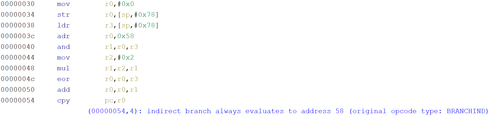
Here's a snippet of the obfuscated ARM code:

The comments off to the side indicate the values of the registers and memory locations as the code executes. Basically, through a convoluted series of arithmetic operations, R0 ultimately obtains the value 0x8E8C, which is then moved into the program counter (PC register) on the final line. All of this code is effectively just a branch to loc_8E8C. However, due to the obfuscated implementation, most disassembler tools won't be able to determine the branch destination, and hence will simply stop disassembling after the line ending in -88. The Hex-Rays decompiler can successfully resolve this branch, but chokes on the next one:

(In fairness to Hex-Rays, if the user manually adds a cross-reference from the final instruction to the resolved destination, it will be able to proceed with decompiling the code at the target address. The analysis described herein can furnish such branch targets.)
This is another form of obfuscation that can be handled by the analysis described by this entry. Similarly to the steps given previously, import the binary "ARM-LE-32-v8-Default.bin" into your Ghidra project. This time, for the "Language", select "ARM / v8 / 32-bit / little-endian / default", as in:

As before, upon loading, Ghidra will prompt you whether you would like to analyze the binary. Select 'Yes'. Next, under the Script Manager window, in the “Deobfuscation” directory, run "Example2ARM.java". By default, the script will add comments to the disassembly listing when it resolves conditional or indirect branches. In particular, running the script should add the comment shown in the figure below:
Let's also take a look at some other output options. For both this example and the previous one, I have shown assembly snippets with manually-written comments suggesting what the written values look like. In fact, given that the analysis automatically computes such information, we don't have to manually create comments like these. Towards the bottom of Example2ARM.java, you will see four calls to "runWithAnalysisOptions", where the first one is enabled and the final three are commented out. Uncomment the second one (the one with "ValueComments" in the code) and run the script again. After adjusting Ghidra's listing fields in the Jenga display (namely, enabling the "PCode" field, and dragging the "Post-Comments" field next to it), we get a nice listing showing the three-valued quantities derived by the analysis after every pcode operation, as such:

Notice that many values have been determined to be fully constant. In fact, every pcode operation in this example either produces a value that is fully known (i.e., all constant bits), or fully unknown (i.e., all unknown bits). For example, take a look at the output for the pcode in the first instruction, which I've reproduced below for easier discussion:
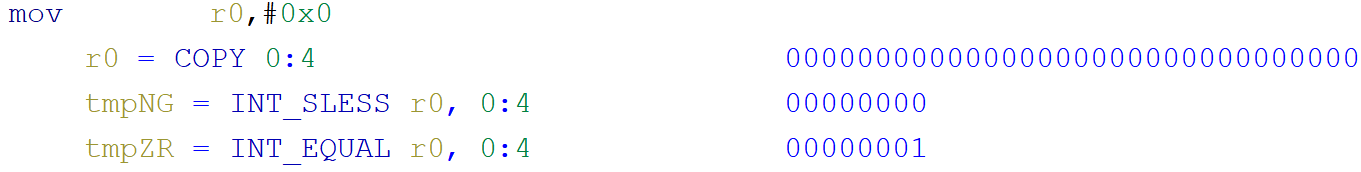
The second pcode line computes whether the register "r0" is signed less-than 0, and stores the boolean result in a variable named "tmpNG". Since the value of r0 was determined to be 0, the result of this comparison is known: 0 is in fact not less than 0, so the value written to tmpNG is 0. Similarly, the subsequent line compares r0 against 0 for equality, and sets the variable "tmpZR" based on the result. Since r0 contains 0, tmpZR will always be 1 after this comparison.
In compiler theory, an analysis known as "constant propagation" determines when variables are known to contain constant values at a given point in the program, and replaces the variable with the constant. A related analysis, "constant folding", determines when all of the inputs to a given operator are constant values (such as the signed less-than operator, or equality comparison operator from the code just discussed), computes the constant result, and replaces the operation with its result. Our analysis performs both constant propagation and constant folding as a side-effect of its main goal. Also, the code optionally has the ability to modify the pcode along those same lines.
Modify the "Example2ARM.java" script again, this time uncommenting the third call to runWithAnalysisOptions (the one with "PcodeComments" in the code), and commenting out the others. Now, run the script. Below is an example of its output for the same truncated example above. I have manually indicated with red dots where the analysis has changed the pcode -- namely, the computations for "tmpNG" and "tmpZR" both become "COPY" operations, instead of their original "INT_SLESS" and "INT_EQUAL" operations.

(The output may be a bit difficult to read -- it uses the so-called "raw" output for the pcode, which differs from the output that Ghidra uses by default.) For completeness, here are the analysis results for the entire sequence.

Example #3: Virtualization Obfuscation
The previous two examples were mostly for proof of concept. We isolated two representative examples of the opaque predicates generated by the respective obfuscators, and demonstrated that the analysis is capable of resolving the correct branch destinations. Though both examples came from real-world scenarios, they were curated for the sake of demonstrating the analysis. For this example, we will use a real-world sample, unmodified, in its natural habitat.
The sample in question is a purportedly malicious binary, obtained from VirusTotal, which is protected by a virtualization obfuscator. (I haven't analyzed the sample and can't speak about its malicious activities.) Rather than examining sample snippets as in the previous two examples, we shall compute an analysis across entire control flow graphs, taking branches into account. The control flow graph-based analysis is computed very much in the same style as so-called "global intraprocedural dataflow analyses" from compiler theory.
The sample can be found in the same directory as the previous examples. It is contained in a .ZIP file with the password “infected”. Extract this archive to a location that won’t be intercepted by your anti-virus software.
The VM uses a similar type of obfuscation as we've already seen -- fake branches based upon constant values -- though the implementation is distinct from the previous examples. Here's a representative example of one of its opaque predicates:

The middle basic block begins by setting CH to 55h. Next, the code subtracts 0Ch from CH. After an unimportant unconditional branch, it then performs a "JO" conditional branch, which is taken if the OF flag had been set by the subtraction. Since the values just described are all constants, the branch has to evaluate the same way every time it executes -- it will either always be taken, or never be taken. (In fact, it can never be taken.)
The analysis library contains one final result visualization technique not described by the examples above. When the analysis determines that a branch always goes in one direction, as long as the code down the not-taken path is not referenced elsewhere, we can color the not-taken instructions in red. Then, in concert with Ghidra's "Window->Function Graph" visualizer, we can easily visualize which parts of the code were not executed. In the figure below, the blue nodes were executed, but the red nodes were not. You can reproduce this for yourself by running the Example3VM.java script.

Problem: Parity Flag
At this point in the blog entry, it should not be surprising that we can detect these opaque predicates and remove them. I did run into one snag trying to use Ghidra on this sample. Namely, some of the opaque predicates are based on the x86 parity flag:

However, by default, Ghidra's x86 language model does not model the updates to this flag. That is to say, even if an x86 instruction modifies the parity flag, Ghidra's pcode translations do not include updates to this register. For example, both the AND and OR instructions in the snippet below do in fact set the parity flag when executed on an x86 processor. However, as you can see, the pcode does not contain updates to the parity flag.

Although this is a sensible design choice for many binary program analyses, we find ourselves in need of such information. For most binary analysis tools, we would find ourselves somewhere between screwed with no way to proceed at one extreme, or facing a non-trivial development effort to model the parity flag at the other. With Ghidra, I managed to solve the issue within about a half an hour. More specifically, under the Ghidra installation, the file ./Ghidra/Processors/x86/data/languages/ia.sinc contains the following snippet:

I was able to simply insert code to properly model the parity flag (the diff is here). After reloading the binary, now the pcode contains proper updates to the parity flags:

I was very impressed at how easy it was to enable this change. Between that and the fact that my analysis worked out of the box on ARM, Ghidra has proven itself to be very capable in the binary program analysis department, not a curiosity or a toy.
Control Flow Graphs
The virtualization obfuscator employed by this binary obfuscates the VM instruction handlers with opaque predicates as demonstrated above. Most unobfuscated handlers, in reality, consist of a single basic block with no control flow. However, a few of the handlers do contain legitimate control flow, including one with a loop. We would like to remove bogus control flow, while at the same time respecting the legitimate control flow.
Rather than hacking together a proof of concept that would only serve as a demonstration, I decided to solve this problem the proper way. In particular, I implemented a library for representing and creating control flow graphs, which is configurable in a variety of ways. Then, I implemented the classical compiler algorithm for solving forward data flow analysis instances. (At present, this code is specialized for the analysis described hereinbefore, but I will likely generalize it to support arbitrary forward and backward data flow problems on pcode control flow graphs). This involved a non-trivial development effort that accounts for over 30% of the code at present.
A False Negative
As one final curiosity, I'll present an example where the analysis was not sophisticated enough to resolve one particular opaque predicate. Take a look at the graph below.

The first assembly language instruction in the first block actually expands into a loop in the pcode control flow graph, which results in complete loss of information about the memory contents. The second, red-underlined line adds a value from memory to the ESP register. Given that the memory state is unknown at this point, the value being added to ESP is unknown, hence the entire register ESP is unknown. Therefore, the subsequent instructions that access the stack are doing so at unknown addresses, so we can't model their effects precisely. As a result, although the third basic block implements a typical opaque predicate that we would ordinarily be able to resolve, because it involves the stack, our analysis cannot resolve it.
So be it. Actually, this is the only opaque predicate in the whole binary that the analysis is unable to resolve.
Conclusion
This blog entry served to announce the release of an open-source deobfuscation plugin for Ghidra. In actuality, this is part of a larger effort, unimaginatively termed "GhidraPAL", short for Ghidra Program Analysis Library. Of the four packages in the distribution at present, three of them are generic and are not tied to the analysis described in this entry. I plan to implement more standard functionality in the future (such as integration with SMT solvers), as well as any other analysis I find useful in binary analysis, and of course weird research efforts that may or may not be useful.
I still have one more thing to tackle before I feel comfortable recommending Ghidra wholeheartedly for automated binary program analysis. If it turns out that, as usual, I am just being neurotic and anticipating problems that will in fact not materialize, then I'll give it my fullest blessing. For now, my experience with this project was almost entirely painless. Ghidra's API is, on the whole, absurdly well-documented. At times I found myself griping that I couldn't find things because there was too much documentation. (Imagine that as a complaint about a software system.) Beyond the documentation, it's also sensibly designed, and includes a lot of very useful functionality in the standard distribution. For classical data flow analysis and abstract interpretation, I highly recommend it, though the jury is still out on SMT integration.